The toolbar is very similar to Microsoft Office Excel.
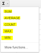
A function will calculate numbers for you automatically. On the toolbar you click on the sigma symbol. Then you select the list of numbers you would like to use in the formula.
SUM- total list
AVERAGE- mean of list
COUNT- number of items in list
MAX- maximum number in list
MIN- minimum number in list

When inserting an image you have several options. You can upload an image from your documents, take a snapshot, insert an image from a website, upload an image from your Google Drive or search for an image in Google.
When inserting a chart, you must select the data you are wanting to use. You have many charts options and settings to use. If you do not like the recommendations, you can choose other types under Chart types. You can also customize your chart by clicking on customizations. That is where you can change color and font, add a titles, add labels to your axis and many more options for your chart. Once you have finish you click done, and the chart will show to the right of your data.


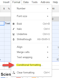
For example, if you want the failing grades to show up in red and the 70-75 grades in pink.
Depending on the numbers, your data will change as new number or calculations are inserted in your Google Sheet.
To get an add-on you will need to get to "Add-on" and then "Get add-ons".
This add-on created awesome 3D charts, graphs and more. It adds bold colors and multidimensional to the chart or graph.
This add-on allows you to plot your data on a map. If you have a list of addresses in a Sheet, this add-on will map it on Google Maps.
This add-on converts any Google Sheet into a Google Doc.


